Introduction:
The UW system is curious in determining whether or not certain factors influence the amount of enrollment at two different schools, the University of Wisconsin Milwaukee and the University of Wisconsin Eau Claire. The amount of enrollment at each university may be influenced by factors such as the amount of income and education in certain counties, as well as the distance of each county away from each university. These variables can determine a student’s decision in deciding between different universities, thus affecting the amount of enrollment at different schools. Data regarding the enrollment amount at each university as well as income, percent bachelor’s degree, and distance for each county in Wisconsin is used. In order to determine whether or not these variables influence the amount of enrollment the data is analyzed using regression analysis. After performing regression analysis on the data the UW System can determine which factors are most significant in influencing enrollment amounts at the University of Wisconsin Milwaukee and the University Wisconsin Eau Claire. When significant factors are determined, spatial representations are used in relation to the regression statistics to determine spatial patterns of enrollment based on the most influential variables.
Methodology:
Regression analysis will determine whether or not to reject the null hypothesis, stating that there is no relationship between each variable and enrollment at both universities. If statistically significant, then the alternative hypothesis, stating there is a linear relationship between each variable and enrollment at both universities, can be investigated. In order to properly determine which variables have the most significant influence on the amount of enrollment at each university the data is analyzed through regression analysis in SPSS. Regression analysis statistics are performed in SPSS to determine whether or not any of the three suspected variables have a significant relationship to the amount of enrollment at each university. Six different regression analyses are performed using the enrollment data for both universities in relation to each of the three variables. The results each analysis will indicate which variables have significant relationships to the amount of enrollment at each university, thus indicating which factors are more influential on a student’s decision to attended different universities.
The data for the three variables include median household income in each county, percent bachelor’s degrees in each county, and the distance of each county (from its center) away from each university. The data regarding median household income and percent bachelor’s degree for each county are ready for analysis and do not need to be normalized or altered. However, the distance data must be normalized based on the population for a more accurate analysis of the data. This is done by dividing the distance for each county by the population for each county. The normalized distance data will be used in the regression analysis.
Three separate regression analyses are performed using the enrollment data for the University of Wisconsin Eau Claire in relation to each of the three variables. The regression analysis will indicate whether or not there is a relationship between each variable and the enrollment amount at Eau Claire as well as create an equation of the relationship providing a means to make predications regarding that relationship. The goal is to establish whether or not the enrollment amount at the university depends on variables such as income, percent bachelor’s degrees, and distance. Because of this the enrollment data for this university is used consistently as the dependent variable in order to determine how the other variables, the independent variables, influence enrollment amount. After three separate regression analyses were performed comparing the University of Wisconsin Eau Claire enrollment data to the suspected independent variables, the same was done using the University of Milwaukee enrollment data compared to the same three independent variables. The results of each regression analyses in SPSS will indicate which variables have a significant relationship with the enrollment amounts at each university as well as the pattern of that relationship in the form of an equation.
After the regression analysis provides the statistics determining the most significant variables, the data for those variables can be graphed in relation to the enrollment data for each university. The graphs will provide a visual interpretation of the trends associated with each significant variable. A scatterplot will display the actual pattern of the raw data in comparison to a trend line with an equation determined by regression analysis. The observed data plotted in comparison to a trend line representing the predicted relationship helps to visually identify both the pattern and strength associated with the relationship of a given variable with the amount of enrollment at both universities.
In order to better understand the most influential factors, spatial representations of each significant variable are produced to be examined in relation to the regression statistics. The spatial representations map the residuals of the statistically significant variables. The residuals indicate the amount the actual data deviates from the predicted value of the relationship provided by the equation. Residuals that are closer to zero indicate no deviation of the actual data to the predicted outcome, meaning a relationship between variables can be accurately predicted. The further the residual is from zero in either direction indicates a less accurate prediction of a relationship. The residuals for each county for the significant variables can be saved in SPSS during regression analysis to be used in ArcMap. The maps created in ArcMap of the residuals help identify which counties in Wisconsin are accurate representations of specific factors influencing enrollment at each university, and which counties appear as outliers. Establishing areas where outliers are occurring allows for a clearer interpretation of certain patterns regarding the influence of specific factors on enrollment at each university.
Results:Based on the results of the regression analyses comparing the Enrollment amount at the University Wisconsin Eau Claire and each of the three variables, two of the three variables were found to be statistically significant. The null hypothesis is rejected regarding both percent bachelor degrees and the distance variable. Therefore, there is a significant linear association between percent bachelor’s degrees and Eau Claire enrollment as well a significant relationship between distance and enrollment. The null hypothesis is rejected for both these variables considering the regression analysis provided statistics with a significance level below 0.05. However, the variable regarding income did not show a significant association to enrollment at Eau Claire after regression analysis. A significance level for this variable greater than 0.05 fails to reject the null hypothesis, meaning there is not a significant linear relationship between median house hold income and Eau Claire enrollment.

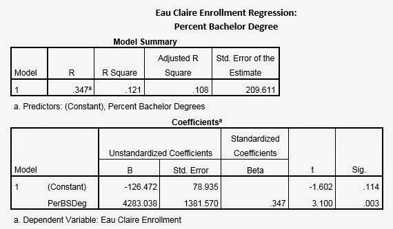

After establishing which variables are significant in regards to influencing enrollment at Eau Claire, further analysis of the regression statistics provides information about the strength and direction of that relationship. In regards to the influence of percent bachelor’s degrees on Eau Claire enrollment, the relationship provided by an equation of Y=-126.472+4283.038X and an R2 of 0.121 indicates a weak but apparent positive linear association. Thus, for every one increase in percentage of bachelor’s degrees enrollment at Eau Claire increases by approximately 43 students. However, even though the relationship is proved to be statistically significant the predictions that can be made provided by this equation are fairly inaccurate considering the R2 of 0.121 is relatively low, representing a weak relationship. On the other hand, the distance variable not only proves to be statistically significant, but the relationship between distance and enrollment is much stronger. The equation of Y=8.518+0.124X and an R2 value of 0.945 indicates a strong positive relationship between the two variables. As the distance increases, enrollment in turn increases at a rate of 0.124. Where counties 500 miles away have a typical enrollment of 70 students at Eau Claire. Predications that are made using the equation for this variable are fairly accurate considering the strong relationship provided by the R2 value of almost 0.945, but the rate of increase is fairly minimal.


Based on the results of the regression analyses comparing enrollment amounts at the University of Wisconsin Milwaukee and each of the variables, all three of the variables were proved to be statistically significant. Because of a given significance level of less than 0.05 in all the results we can reject the null hypothesis concerning all three variables. Therefore, there is linear association between Milwaukee enrollment and distance, as well as linear relationship between Milwaukee enrollment and both percent bachelor’s degrees and income. Despite the relevance of all three variables being statistically significant, the strength and pattern concerning each relationship still needs to be examined.


The relationship between median house hold income and Milwaukee enrollment is the weakest of the three relationships. The equation of Y=-1006.75+0.039X created through regression analysis displays a positive linear relationship between income and enrollment. For every increase in median house hold income, enrollment increases by 0.039. A median household income of around 30,000 for a county contributes to about 164 students at Milwaukee. Despite the ability to make predictions of the influence of income on enrollment using the equation, the R2 value of 0.068 indicates a very weak relationship between the variables making predictions less accurate. The relationship concerning the influence of percent bachelor’s degrees on Milwaukee enrollment shows a slightly stronger relationship. Although the relationship between the variables is slightly stronger than the last, it is still fairly weak as indicated by an R2 value of 0.16. The equation of Y=-1082.762+24556.66X explains a positive linear relationship, where for every one percentage increase in the amount of bachelor’s degrees, enrollment increases by about 245 students. Predictions made from this equation will likely be inaccurate concerning the weak relationship between the variables. However, the relationship regarding the influence of distance on enrollment at Milwaukee has a much stronger linear association. The R2 value of 0.922 identifies a strong association between the variables and the equation of Y=108.041+0.015X shows a positive relationship. For counties 500 miles away there is an enrollment of 115 student and is increasing by 0.015 students per mile away. Predictions concerning the influence of distance on Milwaukee enrollment are fairly accurate taking into consideration the overall strength of the relationship, however the rate of increase of enrollment per increase in distance in minimal.


Further connections can be made when results of the regression analyses are considered in relation to the spatial representations of the residuals for the significant variables. The areas on the maps that display residuals further away from zero can be determined as outliers, meaning those are areas that do not follow the expected prediction given by the equations.

The maps on the bottom are displays the residuals of the relationship between the University of Wisconsin Milwaukee and each of the three significant factors. The map on the bottom right shows the residuals of the relationship between percent bachelor’s degrees and enrollment. In this map, the residuals in green are the ones closest to zero making those counties ones that are accurate predictions of the influence of bachelor degrees. The light blue counties, like the green, are also fairly accurate. However, the counties in dark blue and yellow are the counties where the percent bachelor’s degrees do not provide an accurate representation of the enrollment at Milwaukee, and that the influence of bachelor’s degrees in these areas is not as strong. The map in the center portrays the residuals of the relationship between distance and Milwaukee enrollment. Majority of the state, shown in yellow, follow the predicted pattern of the influence of distance on enrollment considering those are the counties with residuals closet to zero. There are a select few counties, particularly the ones in blue, with residuals much higher than zero, meaning distance in not a significant influence in those areas and cannot be used to accurately determine enrollment. The last map shows the residuals for the relationship between income and enrollment. Much of the map, in green and some yellow, indicate that income is a predictable factor of influence for determining enrollment in those counties. There are, however, a couple of outliers in blue indicating income is not an influential factor contributing to Milwaukee enrollment.
Conclusion: When considering the statistics as well as the residual maps conclusions can be made about influential factors determining enrollment at different schools. Not only can the statistics determine which factors are statistically significant and have the most influence but they also provide information concerning the pattern and strength of the influence. This information is particularly helpful when used in relation to the residual maps, as certain significant factors of influence vary based on location. Overall, the statistics can provide the means to determine which factors are most influential, but the maps allow clearer interpretation of where each variable has the most influence. Some factors deemed the most influential in determining enrollment at different schools are more significant in some counties compared to others. Because of this different areas seem to be more influenced by one variable, and may not be as influenced by another.
The most significant factors influencing enrollment at the University of Eau Claire include the percentage of bachelor’s degrees in each county as well the distance away from the university. Even though both of these factors have a statistically significant relationship with the amount of enrollment, the influence varies on a county level. When considering the influence of the percent bachelor’s degrees it is clear that much of the state follows the predicted pattern associated with the relationship to enrollment. Thus, much of these areas indicate that the amount of bachelor’s degrees has a predictable influence on enrollment. However, certain areas in the center of the state along with a few counties to the north do not follow the predicated relationship between bachelor degrees and enrollment. Because of this the influence of the amount of bachelor’s degrees on enrollment is not as strong in these areas. In contrast, the same counties, along with a few others, are clearly influenced by distance and have a strong connection to the pattern associated with the relationship between distance and enrollment. Coincidentally much of the counties that follow this pattern are near the University of Wisconsin Eau Claire, therefore it is not surprising to conclude distance is an influential factor in these areas.
The most significant factors which influence the enrollment at the University of Wisconsin Milwaukee include, percentage of bachelor’s degrees in each county, the median income in each county, as well as distance away from the university. Much of the state is equally influenced by percentage of bachelor’s degrees in the sense that most counties follow the pattern associate with the relationship, as shown by the residual map. However, Milwaukee County does not follow the same pattern as the rest of the state, where the influence of bachelor’s degrees on enrollment is minimal, and that other factors have much more influence in this county. Similar the lack of influence associated with bachelor’s degrees on enrollment in Milwaukee County, income is another factor that is not as influential. Much of the rest of the state has a predictable enrollment amount associated with the influence of income, however Milwaukee County does not. The influence of distance in Milwaukee County, on the other hand, appears to be the most predictable influence on enrollment.
Based on analysis of all the data, it is easy to determine that the most significant factor influencing enrollment at both university is distance. When considering how other significant factors influence enrollment at each university, the influence is not the same throughout the state. While some counties may be more influenced by the percentage of bachelor’s degrees other counties, specifically the ones closer to the university, are more influenced by distance.
No comments:
Post a Comment